1 Introduction
This vignette provides a concise, runnable introduction to using pviem to estimate population immunity to poliovirus in Fakeland, a fictional demo country with synthetic example data included in the package. It walks through a minimal end-to-end workflow: configuration, data preparation, sampling-based immunity estimation, and summarization/visualization. If this is your first time using the package, read vignette("setup") to configure it and vignette("data") to learn about required inputs. For complete examples, see vignette("workflow").
2 Quick workflow
At a high level the workflow is:
- Configure the package with
config_pviem(). - Load and preprocess input datasets (vaccination schedules, efficacy, routine immunization, births, spatial neighbors).
- Generate stochastic immunity samples with
compute_immunity_samples(). - Summarize samples (point estimates and uncertainty) with
summarize_immunity_samples()and visualize results.
2.1 Setup
alpha_ <- 0.5
imm_color_scheme <- c(
  mucosal = "#0072B2",
  humoral = "#D55E00"
  # mucosal = "#66a61e",
  # humoral = "#7570b3"
)
config_pviem(
  admin = c("prov_code", "dist_code"),
  year = "year",
  month = "month",
  birth = "live_births",
  monthly = FALSE
)
2.2 Load and validate data
# Vaccination schedule and efficacy estimates
vs_table <- preprocess_vs_info(dummy_vs_info)
efficacy <- preprocess_efficacy(efficacy_default, vs_table)

# Routine immunization and birth data
ri_data <- dummy_yearly_ri_data
birth_seasonality <- dummy_birth_seasonality

# Spatial neighbors
neighbors <- get_neighbors(
  fakeland,
  admin_cols = c("admin1_code", "admin2_code")
)

# Sample pair for imputation (target and reference columns)
sample_pair <- get_default_sample_pair(ri_data)

# Vaccine immunity types (customize as needed)
vaccine_immunity_type <- list(
  OPV = c("mucosal", "humoral"),
  IPV = "humoral"
)

# Validate all inputs
validate_all_data(
  vs_info = vs_table,
  efficacy = efficacy,
  ri_data = ri_data,
  birth_seasonality = birth_seasonality,
  sample_pair = sample_pair,
  vax_imm_type = vaccine_immunity_type
)
2.3 Compute immunity samples
Compute stochastic samples that propagate data uncertainty (bootstrapped imputations for missing RI doses). Adjust sampling and imputation modes as needed for reproducibility and speed.
immunity_samples <- compute_immunity_samples(
  n_samples = 5,
  ri_data = ri_data,
  vs_info = vs_table,
  efficacy = efficacy,
  birth_seasonality = birth_seasonality,
  neighbors = neighbors,
  sample_pair = sample_pair,
  imputation_mode = "stochastic",
  sample_mode = "uniform",
  shift_mode = "full",
  hed_assumption = "redistribute",
  max_level = 4,
  dd_assumption = "organised",
  vax_imm_type = vaccine_immunity_type,
  rho = 0,
  per_imm_type = TRUE,
  quiet = TRUE,
  seed = 42
)
2.4 Summarize and visualize
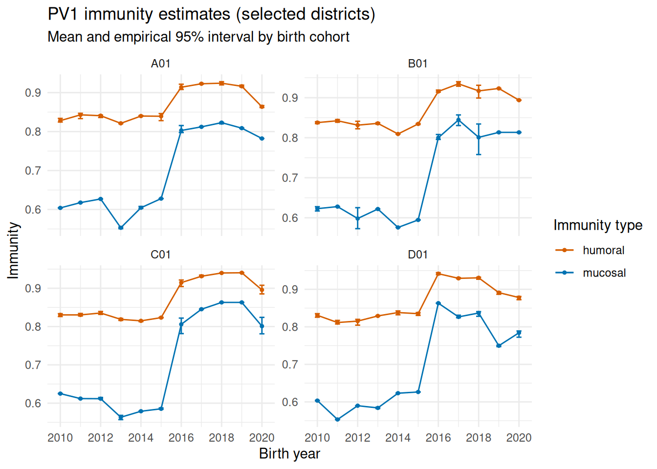
Summarize samples to obtain means and empirical uncertainty intervals at district or province level, then plot birth-cohort trajectories. The example uses only five samples to keep the vignette fast; use many more samples for stable uncertainty estimates in a real analysis.
district_immunity <- summarize_immunity_samples(immunity_samples)
head(district_immunity, n = 10)| prov_code | dist_code | year | serotype | type | .mean | .sd | .median | .lower | .upper | .ci95l | .ci95u |
|---|---|---|---|---|---|---|---|---|---|---|---|
| PR_F | F03 | 2011 | PV1 | humoral | 0.8267057 | 0.0034429 | 0.8247088 | 0.8239099 | 0.8316492 | 0.8224308 | 0.8309807 |
| PR_C | C04 | 2014 | PV1 | humoral | 0.8493411 | 0.0000127 | 0.8493430 | 0.8493261 | 0.8493565 | 0.8493253 | 0.8493569 |
| PR_D | D02 | 2014 | PV1 | humoral | 0.8223947 | 0.0003969 | 0.8224044 | 0.8220055 | 0.8229636 | 0.8219019 | 0.8228876 |
| PR_F | F03 | 2016 | PV1 | humoral | 0.9046483 | 0.0026193 | 0.9057230 | 0.9017938 | 0.9072769 | 0.9013960 | 0.9079005 |
| PR_A | A05 | 2010 | PV1 | humoral | 0.8063637 | 0.0072310 | 0.8094095 | 0.7983127 | 0.8127033 | 0.7973852 | 0.8153422 |
| PR_C | C05 | 2019 | PV1 | humoral | 0.9072122 | 0.0007337 | 0.9071548 | 0.9064349 | 0.9082451 | 0.9063011 | 0.9081232 |
| PR_A | A08 | 2012 | PV1 | humoral | 0.8419114 | 0.0017766 | 0.8431935 | 0.8396794 | 0.8431935 | 0.8397054 | 0.8441174 |
| PR_A | A01 | 2017 | PV1 | humoral | 0.9228570 | 0.0008005 | 0.9231387 | 0.9218252 | 0.9236481 | 0.9218630 | 0.9238510 |
| PR_E | E04 | 2012 | PV1 | humoral | 0.8279406 | 0.0064814 | 0.8248625 | 0.8209580 | 0.8349543 | 0.8198929 | 0.8359883 |
| PR_A | A01 | 2014 | PV1 | humoral | 0.8398836 | 0.0008902 | 0.8395847 | 0.8392622 | 0.8412718 | 0.8387782 | 0.8409890 |
district_immunity[
  dist_code %in% c("A01", "B01", "C01", "D01") & serotype == "PV1"
] |>
  ggplot(aes(x = year, y = .mean, ymin = .lower, ymax = .upper, color = type, fill = type)) +
  geom_line() +
  geom_point(size = .9) +
  geom_errorbar(width = 0.25) +
  facet_wrap(~dist_code, scales = "free_y") +
  scale_x_continuous(breaks = scales::breaks_width(2)) +
  scale_color_manual(values = imm_color_scheme) +
  scale_fill_manual(values = imm_color_scheme) +
  theme_minimal() +
  labs(
    title = "PV1 immunity estimates (selected districts)",
    subtitle = "Mean and empirical 95% interval by birth cohort",
    x = "Birth year",
    y = "Immunity",
    color = "Immunity type",
    fill = "Immunity type"
  )
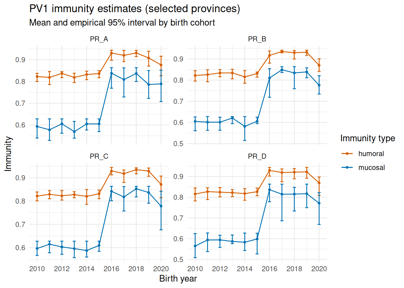
Summarize at province level:
province_immunity <- summarize_immunity_samples(immunity_samples, by_admin = "prov_code")
head(province_immunity, n = 10)| prov_code | year | serotype | type | .mean | .sd | .median | .lower | .upper | .ci95l | .ci95u |
|---|---|---|---|---|---|---|---|---|---|---|
| PR_F | 2011 | PV1 | humoral | 0.8317052 | 0.0087331 | 0.8275144 | 0.8209752 | 0.8440216 | 0.8276180 | 0.8357924 |
| PR_C | 2014 | PV1 | humoral | 0.8200993 | 0.0184905 | 0.8161979 | 0.7861167 | 0.8493494 | 0.8137476 | 0.8264510 |
| PR_D | 2014 | PV1 | humoral | 0.8176770 | 0.0153878 | 0.8224044 | 0.7856410 | 0.8414530 | 0.8130540 | 0.8223000 |
| PR_F | 2016 | PV1 | humoral | 0.9240966 | 0.0139171 | 0.9262625 | 0.9018481 | 0.9387131 | 0.9175832 | 0.9306100 |
| PR_A | 2010 | PV1 | humoral | 0.8226061 | 0.0104477 | 0.8250545 | 0.7997343 | 0.8374451 | 0.8194673 | 0.8257450 |
| PR_C | 2019 | PV1 | humoral | 0.9288427 | 0.0142082 | 0.9378124 | 0.9062157 | 0.9417388 | 0.9239620 | 0.9337234 |
| PR_A | 2012 | PV1 | humoral | 0.8370207 | 0.0070547 | 0.8393857 | 0.8174550 | 0.8451526 | 0.8349013 | 0.8391402 |
| PR_A | 2017 | PV1 | humoral | 0.9199386 | 0.0177892 | 0.9217745 | 0.8912850 | 0.9429963 | 0.9145941 | 0.9252831 |
| PR_E | 2012 | PV1 | humoral | 0.8243528 | 0.0098783 | 0.8258598 | 0.8042737 | 0.8373008 | 0.8202752 | 0.8284303 |
| PR_A | 2014 | PV1 | humoral | 0.8319115 | 0.0125608 | 0.8363136 | 0.8080841 | 0.8470977 | 0.8281378 | 0.8356851 |
province_immunity[
  prov_code %in% c("PR_A", "PR_B", "PR_C", "PR_D") & serotype == "PV1"
] |>
  ggplot(aes(x = year, y = .mean, ymin = .lower, ymax = .upper, color = type, fill = type)) +
  geom_line() +
  geom_point(size = .9) +
  geom_errorbar(width = 0.25) +
  facet_wrap(~prov_code, scales = "free_y") +
  scale_x_continuous(breaks = scales::breaks_width(2)) +
  scale_color_manual(values = imm_color_scheme) +
  scale_fill_manual(values = imm_color_scheme) +
  theme_minimal() +
  labs(
    title = "PV1 immunity estimates (selected provinces)",
    subtitle = "Mean and empirical 95% interval by birth cohort",
    x = "Birth year",
    y = "Immunity",
    color = "Immunity type",
    fill = "Immunity type"
  )
For production runs, increase n_samples until the summaries are stable and adjust the parallel-processing plan to suit the available hardware.