Polio immunity estimation workflow

1 Introduction

This vignette provides complete, end-to-end worked examples demonstrating how to use the pviem package to estimate vaccine-induced immunity across administrative levels. It shows how data flows through the analysis pipeline from preparation through visualization and advanced customization.

Read these vignettes first (in order):

vignette("setup") — Package configuration and column mapping,
vignette("data") — Data formats, structures, and validation,
vignette("pviem") — Minimal quick-start example.

This vignette builds on those foundations with practical end-to-end examples, advanced workflows, visualization techniques, and customization patterns.

Note

This vignette uses synthetic data for a fictional country called Fakeland (available as fakeland in the package). All analyses are illustrative only and should not inform real-world decision making.

2 Setup

Load required packages and configure parallel processing:

library(pviem)
library(dplyr)
library(tidyr)
library(ggplot2)
library(furrr)

# Configure parallel processing (adjust workers for your system)
plan(multisession, workers = min(4L, availableCores()))
seed <- 42
set.seed(seed)

Configure the package (for detailed options, see vignette("setup")):

admin_cols <- c("prov_code", "dist_code")
config_pviem(
  admin = admin_cols,
  year = "year",
  month = "month",
  birth = "live_births",
  monthly = FALSE
)

Define visualization parameters for this workflow:

alpha_ <- 0.5
color_scheme <- c(
  birth = "#8B5CF6",
  known = "#155853",
  imputed = "#b51623",
  shifted = "#383596",
  redist = "#836720",
  low = "#fee5d9",
  high = "#a50f15"
)
imm_color_scheme <- c(
  mucosal = "#0072B2",
  humoral = "#D55E00"
  # mucosal = "#66a61e",
  # humoral = "#7570b3"
)

legend_labels <- c(
  birth = "live births",
  known = "known doses",
  imputed = "imputed doses",
  shifted = "shifted doses",
  redist = "redistributed doses"
)
# Example parameters for later use in the vignette
dose_eg <- "IPV2"
year_eg <- 2010
serotype_eg <- "PV1"

3 Data preparation

The package includes synthetic datasets (prefixed with dummy_*) that demonstrate expected input structures. For comprehensive data format documentation, validation rules, and troubleshooting, see vignette("data").

This section focuses on loading and preprocessing these data within an end-to-end workflow context.

# Vaccination schedule and efficacy estimates
vs_table <- preprocess_vs_info(dummy_vs_info)
efficacy <- preprocess_efficacy(efficacy_default, vs_table)

# Routine immunization and birth data
ri_data <- dummy_yearly_ri_data
birth_seasonality <- dummy_birth_seasonality

# Spatial neighbors
neighbors <- get_neighbors(
  fakeland,
  admin_cols = c("admin1_code", "admin2_code")
)

# Sample pair for imputation (target and reference columns)
sample_pair <- get_default_sample_pair(ri_data)

# Vaccine immunity types (customize as needed)
vaccine_immunity_type <- list(
  OPV = c("mucosal", "humoral"),
  IPV = "humoral"
)

# Validate all inputs
validate_all_data(
  vs_info = vs_table,
  efficacy = efficacy,
  ri_data = ri_data,
  birth_seasonality = birth_seasonality,
  sample_pair = sample_pair,
  vax_imm_type = vaccine_immunity_type
)

# Summary of the RI data
summary(ri_data)
#>      prov_code       dist_code        year           OPV0            OPV1      
#>  Length   :440   Length   :440   Min.   :2010   Min.   :30267   Min.   :25612  
#>  N.unique :  6   N.unique : 40   1st Qu.:2012   1st Qu.:39919   1st Qu.:37891  
#>  N.blank  :  0   N.blank  :  0   Median :2015   Median :46160   Median :44233  
#>  Min.nchar:  4   Min.nchar:  3   Mean   :2015   Mean   :46299   Mean   :44209  
#>  Max.nchar:  4   Max.nchar:  3   3rd Qu.:2018   3rd Qu.:51961   3rd Qu.:49713  
#>                                  Max.   :2020   Max.   :68364   Max.   :67027  
#>                                                 NAs    :47      NAs    :27     
#>       IPV1            IPV2        live_births   
#>  Min.   :29576   Min.   :26912   Min.   :35317  
#>  1st Qu.:40299   1st Qu.:39220   1st Qu.:42260  
#>  Median :46094   Median :44296   Median :49293  
#>  Mean   :46250   Mean   :44806   Mean   :48027  
#>  3rd Qu.:52161   3rd Qu.:50153   3rd Qu.:52476  
#>  Max.   :63323   Max.   :66038   Max.   :61286  
#>  NAs    :98      NAs    :91

# For later use in plotting

## Dose columns
dose_cols <- intersect(names(ri_data), vs_table$dose)

## Get a dist_code which contains NAs
.dcode <- ri_data %>%
  filter(OPV0 < OPV1 | IPV1 < IPV2) %>%
  pivot_longer(
    cols = all_of(dose_cols),
    names_to = "dose",
    values_to = "doses"
  ) %>%
  summarise(num_na = sum(is.na(doses)), .by = dist_code) %>%
  filter(num_na > 0) %>%
  pull(dist_code) %>%
  unique() %>%
  sample(1)

## Corresponding RI data for the selected district (used in later plots)
ri_data_dcode <- ri_data %>%
  filter(dist_code == .dcode) %>%
  pivot_longer(
    cols = all_of(dose_cols),
    names_to = "dose",
    values_to = "doses"
  ) %>%
  left_join(vs_table %>% select(vaccine, dose), by = "dose") %>%
  mutate(
    source = if_else(is.na(doses), "imputed", "known"),
    vaccine = factor(vaccine, levels = unique(vs_table$vaccine))
  ) %>%
  select(all_of(c(admin_cols, "year", "vaccine", "dose", "source")))

4 Immunity estimation workflow

This section provides a comprehensive overview of the methodological steps for estimating population immunity levels. The pipeline comprises several interconnected components, each playing a crucial role in the overall estimation process.

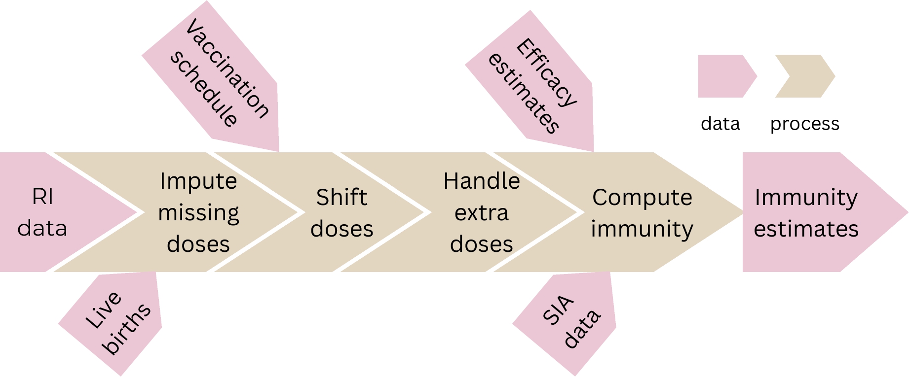
While pviem provides automated functions that handle these steps seamlessly (detailed in Section 4.6), understanding the underlying methodology ensures proper interpretation of results and informed analytical decisions.

The following subsections break down each component with detailed explanations and illustrative examples.

4.1 Imputation process

The imputation process estimates missing values in the routine immunization data, which is crucial for maintaining analytical integrity with incomplete datasets. The impute_missing_doses() function provides three imputation approaches via its imputation_mode argument: stochastic, deterministic, and custom. We will give more details about each later in this section.

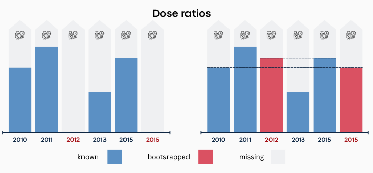
Missing doses are imputed through dose-to-dose ratios rather than directly on dose counts. The ratio is computed by dividing the number of children who received the target dose by the reference dose used as the denominator. For imputation to work properly, both the target and reference doses must have at least one non-missing value in each administrative unit across the available time period.

The selection of a denominator should be guided by known correlations between doses. For example, If children who receive OPV1 are highly likely to receive IPV1 (such as when doses are administered at similar ages), consider using IPV1 as the denominator for OPV1 ratio calculation (and vice versa). The general principle: if you expect a strong correlation between two doses, use them as denominators for each other in ratio calculations.

The pair of columns related to the target and reference in the routine immunization data is defined by the sample_pair argument of impute_missing_doses() function. Helper functions are available to streamline this process:

get_default_sample_pair(): generates the default sample_pair which use live birth as denomintor for doses columns containing missing values;
validate_sample_pair(): validates your custom sample pair format for safety.

4.1.1 Stochastic imputation (bootstrapping)

The stochastic imputation method uses bootstrapping to estimate missing dose values. Bootstrapping is a statistical resampling technique that estimates the distribution of a statistic by sampling with replacement from observed data.

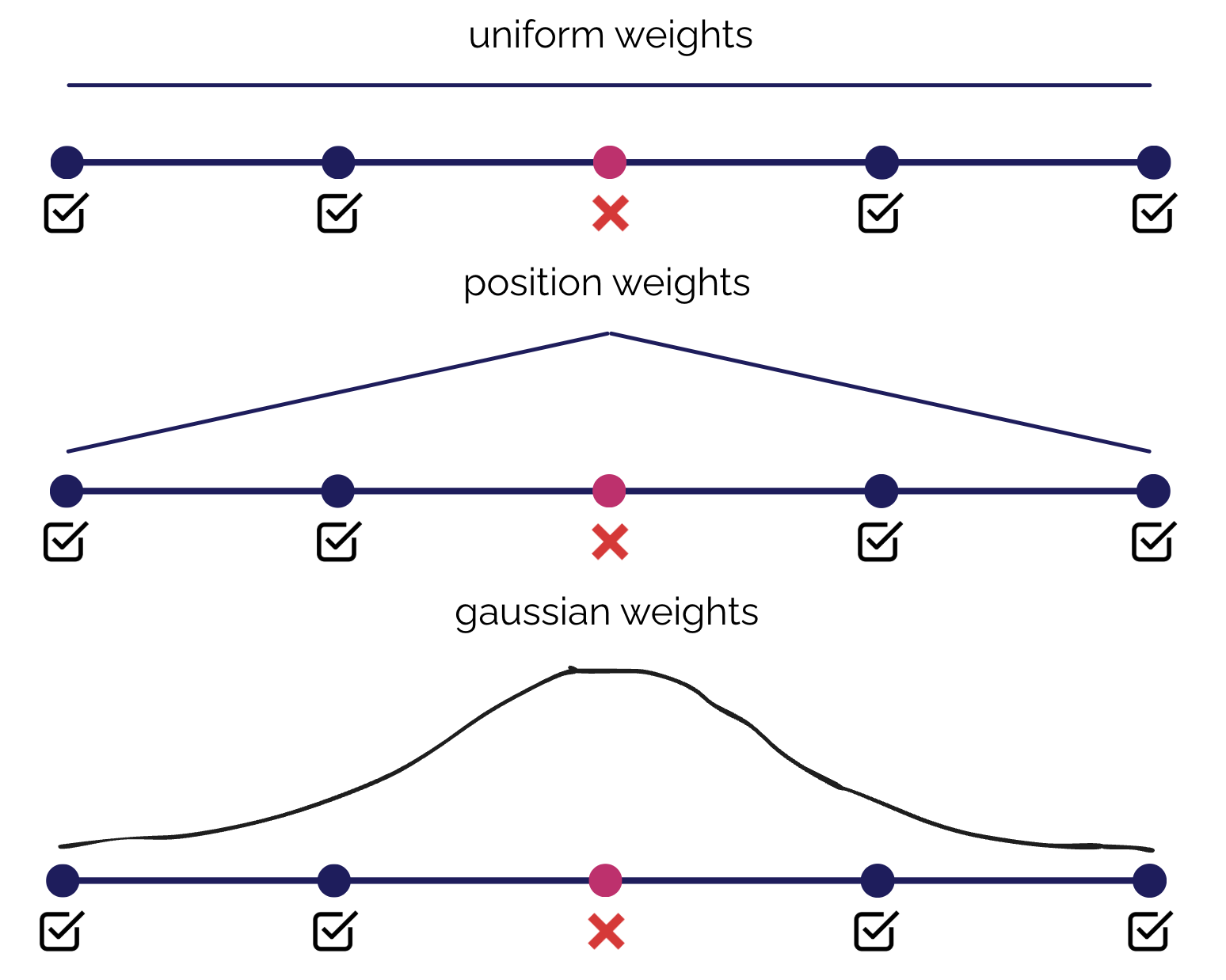
Figure 3: Stchastic imputation (bootstrapping) sampling strategies.

This method offers three sampling strategies via the sample_mode argument, each based on different assumptions as shown on Figure 3:

'uniform': Assumes equal probability of sampling from any non-missing year within a district. All observed years are treated identically regardless of their temporal distance from the missing value.
'position': Assigns higher sampling probability to non-missing values that are temporally closer to the missing year. Observations near the gap receive more weight.
'gaussian': Similar to 'position' but applies a Gaussian-shaped weighting function, providing a smooth decay in probability as temporal distance increases.

The latter two strategies prioritize observations surrounding the missing value, while 'uniform' treats all years equally. Your choice of sampling mode can significantly impact imputation results and should align with your data characteristics and analytical assumptions.

4.1.2 Deterministic imputation

The deterministic imputation method uses aggregation functions to estimate missing dose values. Unlike stochastic methods that introduce randomness, deterministic approaches yield consistent results by applying specific summary statistics to available data. Through the sample_mode argument, you can specify one of four aggregation methods (provided as a character string, not a function):

'mean': Uses the average of non-missing dose ratios
'median': Uses the median of non-missing dose ratios
'min': Uses the minimum of non-missing dose ratios
'max': Uses the maximum of non-missing dose ratios

Each aggregation is performed within each district for each vaccine dose across all available years.

4.1.3 Custom imputation

The custom approach provides flexibility when built-in methods don’t meet your analytical needs. When selecting this mode, sample_mode must be a function with a specific format which details can be found in impute_missing_doses() documentation.

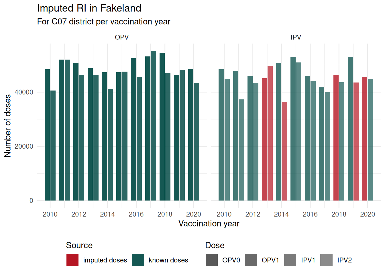
The impute_missing_doses() function generates a new dataset with imputed values. For complete documentation, run ?impute_missing_doses. The code snippet below demonstrates how to use this function.

imputation_mode <- "stochastic"
sample_mode <- "uniform"
# bandwidth <- 1.0 # Used only for the Gaussian sampling mode.

imputed_doses <- impute_missing_doses(
  ri_data = ri_data,
  sample_pair = sample_pair,
  imputation_mode = imputation_mode,
  sample_mode = sample_mode
)
head(imputed_doses, 10)

prov_code	dist_code	year	OPV0	OPV1	IPV1	IPV2	live_births
PR_A	A01	2010	42834	37177	40987	34992	42862
PR_A	A02	2010	34839	31967	42636	40567	39372
PR_A	A03	2010	43223	42298	45736	42955	50237
PR_A	A04	2010	45535	45180	49810	48807	49364
PR_A	A05	2010	48711	45808	47470	46780	51406
PR_A	A06	2010	50235	55359	44519	49800	49454
PR_A	A07	2010	38092	37012	42435	35654	42840
PR_A	A08	2010	40824	36255	33751	31597	36607
PR_A	A09	2010	47222	46390	48236	46122	47975
PR_B	B01	2010	54846	51919	52912	45281	52301

# Check if there is any NA
anyNA(imputed_doses)
#> [1] FALSE

imputed_doses %>%
  filter(dist_code == .dcode) %>%
  pivot_longer(
    cols = all_of(dose_cols),
    names_to = "dose",
    values_to = "doses"
  ) %>%
  left_join(ri_data_dcode, by = c(admin_cols, "year", "dose")) %>%
  mutate(dose = factor(dose, levels = dose_cols)) %>%
  ggplot(aes(x = year, y = doses, alpha = dose, fill = source)) +
  geom_col(position = "dodge2", width = 0.8) +
  facet_wrap(~vaccine, ncol = 2) +
  scale_x_continuous(breaks = scales::breaks_width(2)) +
  scale_fill_manual(
    name = "Source",
    values = color_scheme[c("known", "imputed")],
    labels = legend_labels[c("known", "imputed")]
  ) +
  scale_alpha_ordinal(name = "Dose", range = c(1, 0.7)) +
  guides(
    fill = guide_legend(nrow = 1, byrow = TRUE, title.position = "top"),
    alpha = guide_legend(nrow = 1, byrow = TRUE, title.position = "top")
  ) +
  theme_minimal() +
  theme(legend.position = "bottom", legend.box = "horizontal") +
  labs(
    title = "Imputed RI in Fakeland",
    subtitle = sprintf("For %s district per vaccination year", .dcode),
    x = "Vaccination year",
    y = "Number of doses"
  )

4.2 Dose shifting

The dose shifting process adjusts vaccine dose counts to align with birth cohorts rather than administration years. This alignment is essential because the timing of vaccine administration relative to birth creates a mismatch between the year a child is born and the year their vaccination is recorded.

Why shifting is necessary? Consider a vaccine dose administered at 6 months of age. A child born in January receives this dose in July of the same year, so their vaccination is counted in their birth year. However, a child born in September receives the same dose in March of the following year, meaning their vaccination is recorded in the year after their birth.

To address this temporal misalignment, we shift doses backward proportionally based on the age at administration and the birth seasonality. This process can be visualized in the figure below.

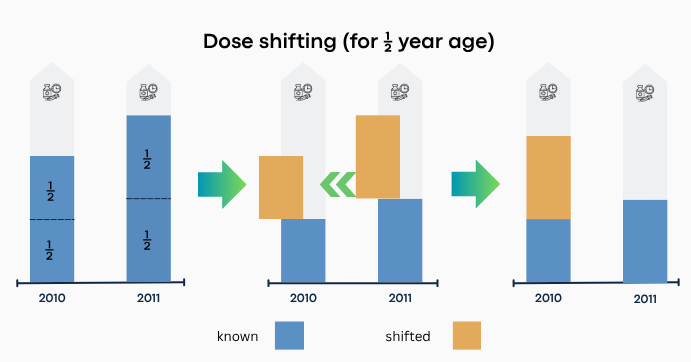
Shifting is based on the proportion of administered doses that should be reassigned for each administrative unit and vaccine dose. This is computed by compute_shift_prop() using the vaccination schedule and, optionally, birth seasonality. When birth seasonality data is not provided, the function assumes a uniform birth distribution across all 12 months. For detailed documentation, run ?compute_shift_prop.

The shift_doses() function performs the actual shifting process, offering three modes via the shift_mode argument: “full”, “partial”, and “random”. Each mode handles the shifting process differently to accommodate various analytical needs. For complete details about each mode, consult the function documentation by running ?shift_doses.

The shift proportion no longer needs to be computed separately and passed to shift_doses(); as of version 0.2.0, it can be calculated directly within the function. Supplying a precomputed shift proportion is still supported.

shifted_doses <- shift_doses(
  ri_data = imputed_doses,
  vs_info = vs_table,
  birth_seasonality = birth_seasonality,
  shift_mode = "full"
)
head(shifted_doses, 10)

prov_code	dist_code	year	IPV1	IPV2	OPV0	OPV1	live_births
PR_A	A01	2010	40926	37791	42834	37403	42862
PR_A	A01	2011	40224	44324	44935	39649	41429
PR_A	A01	2012	39060	47942	43244	43533	43461
PR_A	A01	2013	44230	47778	38402	36817	43097
PR_A	A01	2014	43694	41921	41949	38483	42742
PR_A	A01	2015	41244	40933	45877	44470	43190
PR_A	A01	2016	40900	44378	36508	39623	42730
PR_A	A01	2017	40570	41060	39809	38553	42093
PR_A	A01	2018	37077	40576	39704	34549	41547
PR_A	A01	2019	39411	37449	40268	39689	43123

shifted_doses %>%
  filter(dist_code == .dcode) %>%
  pivot_longer(
    cols = all_of(dose_cols),
    names_to = "dose",
    values_to = "shifted"
  ) %>%
  left_join(ri_data_dcode, by = c(admin_cols, "year", "dose")) %>%
  left_join(
    imputed_doses %>%
      filter(dist_code == .dcode) %>%
      pivot_longer(
        cols = all_of(dose_cols),
        names_to = "dose",
        values_to = "imputed"
      ),
    by = c(admin_cols, "year", "dose")
  ) %>%
  pivot_longer(
    cols = c(imputed, shifted),
    names_to = "source_type",
    values_to = "doses"
  ) %>%
  mutate(
    plot_source = if_else(source_type == "shifted", "shifted", source),
    plot_source = factor(
      plot_source,
      levels = c("known", "imputed", "shifted")
    ),
    dose = factor(dose, levels = dose_cols)
  ) %>%
  ggplot(aes(x = year, y = doses, fill = plot_source)) +
  geom_col(position = "dodge2", width = 0.8) +
  facet_wrap(~dose, ncol = 2) +
  scale_x_continuous(breaks = scales::breaks_width(2)) +
  scale_fill_manual(
    name = "Source",
    values = color_scheme[c("known", "imputed", "shifted")],
    labels = legend_labels[c("known", "imputed", "shifted")]
  ) +
  scale_alpha_ordinal(name = "Dose", range = c(1, 0.7)) +
  guides(
    fill = guide_legend(nrow = 1, byrow = TRUE, title.position = "top"),
    alpha = guide_legend(nrow = 1, byrow = TRUE, title.position = "top")
  ) +
  theme_minimal() +
  theme(legend.position = "bottom", legend.box = "horizontal") +
  labs(
    title = "Shifted vs Imputed RI in Fakeland",
    subtitle = sprintf("For %s district per vaccination year", .dcode),
    x = "Vaccination year for imputed doses / Birth cohort for shifted doses",
    y = "Number of doses"
  )

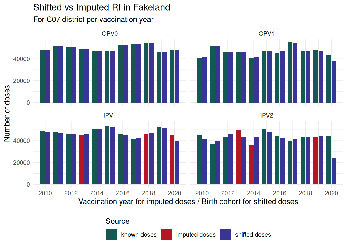
We observe that shifting does not affect birth doses (e.g., OPV0) because those are administered at birth and are already aligned with the birth cohort. Shifting redistributes vaccinations given in later calendar years back into the child’s birth year according to the scheduled age at vaccination and the birth-seasonality profile. Therefore, doses given at older ages are most affected. The impact is strongest at the end of the time series: children born in the most recent years have had less time to receive older-age doses within the observation window, so a larger proportion of those doses is shifted from later years into earlier birth cohorts.

4.3 Handling extra-doses

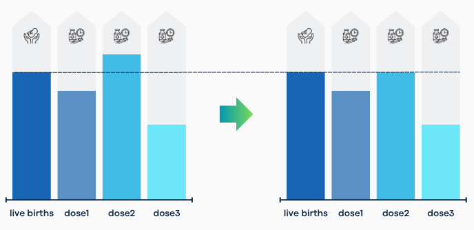
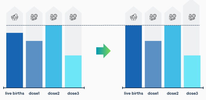
After shifting doses to align with birth cohorts, some districts may show more doses administered than either (i) the number of children who received the preceding dose in the sequence, or (ii) the number of live births in that cohort. Ideally, the number of children receiving the $n^{th}$ dose should not exceed those who received the $(n-1)^{th}$ dose in the same birth cohort. However, discrepancies arise due to factors such as population migration, mortality, data misreporting, or administrative errors. The redistribution process addresses these extra doses under different epidemiological assumptions.

The handle_extra_doses() function implements three scenarios via the hed_assumption argument:

Scenario 1 (“redistribute”): Redistributes extra doses to neighboring districts (see Figure 5). This assumes extra doses primarily result from inter-district migration of children. This is the default scenario.
Scenario 2 (“discard”): Removes extra doses from the dataset (see Figure 5). This assumes extra doses result from overreporting or data quality issues.
Scenario 3 (“scale”): Adjusts live birth counts upward to match the maximum dose count observed across all vaccine doses in each district-year (see Figure 6). This assumes extra doses indicate underreporting of live births.

Figure 5: Handling extra doses process: ‘redistribute’/‘discard’ assumption.

Figure 6: Handling extra doses process: live births scaling (‘scale’ assumption).

When using the “redistribute” assumption, the max_level argument controls how far extra doses can be redistributed, specifying the maximum neighbor distance (in levels of adjacency) to consider. For complete documentation, run ?handle_extra_doses. The code snippet below shows how to use this function:

hed_doses <- handle_extra_doses(
  ri_data = shifted_doses,
  neighbors = neighbors,
  max_level = 4,
  hed_assumption = "redistribute"
)
head(hed_doses, 10)

prov_code	dist_code	year	IPV1	IPV2	OPV0	OPV1	live_births
PR_C	C05	2013	58062	53199	58294	49819	58294
PR_D	D05	2015	41542	38964	43460	42139	43460
PR_F	F03	2017	37559	36549	38996	36357	39924
PR_C	C05	2014	58173	48065	60062	53311	60063
PR_D	D07	2016	49985	49574	50585	47402	50585
PR_B	B02	2012	33450	31288	34088	33446	35587
PR_A	A03	2017	50512	48363	51241	51088	51241
PR_C	C02	2020	49138	26569	54671	42848	54672
PR_E	E03	2010	49975	48685	50973	49467	51252
PR_F	F01	2018	34097	35115	33565	32947	36763

hed_doses %>%
  filter(dist_code == .dcode) %>%
  pivot_longer(
    cols = all_of(dose_cols),
    names_to = "dose",
    values_to = "redist"
  ) %>%
  left_join(
    shifted_doses %>%
      filter(dist_code == .dcode) %>%
      pivot_longer(
        cols = all_of(dose_cols),
        names_to = "dose",
        values_to = "shifted"
      ),
    by = c(admin_cols, "year", "dose", "live_births")
  ) %>%
  pivot_longer(
    cols = c(redist, shifted, live_births),
    names_to = "source",
    values_to = "doses"
  ) %>%
  mutate(
    source = factor(
      if_else(source == "live_births", "birth", source),
      levels = c("birth", "shifted", "redist")
    ),
    dose = factor(dose, levels = dose_cols)
  ) %>%
  ggplot(aes(x = year, y = doses, fill = source)) +
  geom_col(position = "dodge2", width = 0.8) +
  facet_wrap(~dose, ncol = 2) +
  scale_x_continuous(breaks = scales::breaks_width(2)) +
  scale_fill_manual(
    name = "Source",
    values = color_scheme[c("birth", "shifted", "redist")],
    labels = legend_labels[c("birth", "shifted", "redist")]
  ) +
  scale_alpha_ordinal(name = "Dose", range = c(1, 0.7)) +
  guides(
    fill = guide_legend(nrow = 1, byrow = TRUE, title.position = "top"),
    alpha = guide_legend(nrow = 1, byrow = TRUE, title.position = "top")
  ) +
  theme_minimal() +
  theme(legend.position = "bottom", legend.box = "horizontal") +
  labs(
    title = "Live births vs Shifted vs Redistributed RI in Fakeland",
    subtitle = sprintf("For %s district per birth cohort", .dcode),
    x = "Birth cohort",
    y = "Number of doses"
  )

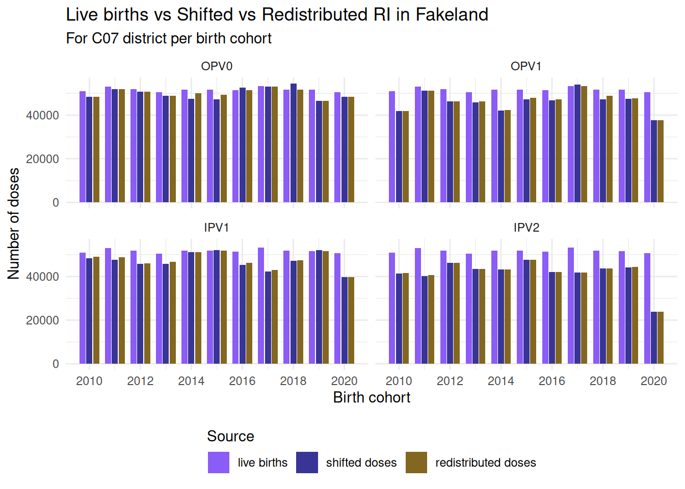
We can see that after redistribution, the number of doses in some districts is reduced to match the number of live births, while in other districts, doses are added to account for the excess in other districts. The impact of redistribution is most pronounced in districts with large discrepancies between shifted doses and live births, often those with significant migration or reporting issues. The “discard” assumption would show a similar pattern but without the addition of doses to neighboring districts, while the “scale” assumption would show an increase in live birth counts rather than adjustments to dose counts.

4.4 Immunity estimation

The immunity estimation process represents the final step in the analytical pipeline, where population immunity levels are calculated based on vaccination coverage data (after redistribution) and vaccine efficacy estimates. This process is performed using the compute_immunity() function. This function implements two approaches via the dd_assumption argument to estimate immunity levels based on different assumptions about dose receipt patterns:

4.4.1 `organised` assumption (default)

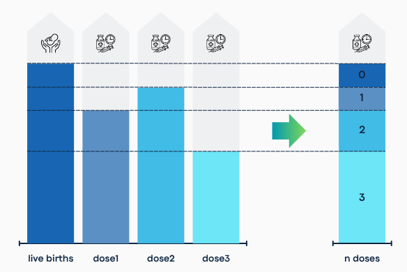
Ideally, the number of children receiving the $n^{th}$ dose of a vaccine in a given district-year should not exceed those who received the $(n-1)^{th}$ dose (or the birth cohort size for first doses). However, real-world data often violates this logical constraint due to migration, mortality, or reporting inconsistencies.

The “organised” assumption enforces sequential consistency in dose receipt and ensures that no child is counted as receiving dose k without having received all preceding doses. The resulting dose-specific populations are then combined with dose-specific efficacy estimates to calculate immunity levels by administrative unit, year, serotype, and vaccine.

Figure 7: The way the number of babies who received exactly n doses is computed.

4.4.2 `random` assumption

This assumption represents a bounding case with extreme assumptions: dose numbers are recorded based solely on the child’s age, independent of vaccination history. Under this scenario, receiving doses at older ages is uncorrelated with receiving doses at younger ages.

Note

This assumption is epidemiologically unlikely and not typically supported by real-world vaccination patterns. It is included primarily as a sensitivity analysis boundary case.

The code snippets below show how to use this function:

immunity <- compute_immunity(
  hed_doses,
  efficacy,
  dd_assumption = "organised"
)
head(immunity, 10)

prov_code	dist_code	year	serotype	vaccine	immunity_level	zero_dose	live_births
PR_C	C05	2013	PV1	IPV	0.5767566	0.0039798	58294
PR_D	D05	2015	PV1	IPV	0.5586908	0.0441325	43460
PR_F	F03	2017	PV1	IPV	0.5581330	0.0592376	39924
PR_C	C05	2014	PV1	IPV	0.5390473	0.0314670	60063
PR_D	D07	2016	PV1	IPV	0.5908520	0.0118612	50585
PR_B	B02	2012	PV1	IPV	0.5487819	0.0600500	35587
PR_A	A03	2017	PV1	IPV	0.5809791	0.0142269	51241
PR_C	C02	2020	PV1	IPV	0.4360651	0.1012218	54672
PR_E	E03	2010	PV1	IPV	0.5787579	0.0249161	51252
PR_F	F01	2018	PV1	IPV	0.5661807	0.0448277	36763

immunity %>%
  filter(dist_code == .dcode) %>%
  ggplot(aes(
    x = year,
    y = immunity_level,
    fill = factor(vaccine, levels = c("OPV", "IPV"))
  )) +
  geom_col(position = "dodge2", width = 0.8) +
  facet_grid(~serotype) +
  scale_x_continuous(breaks = scales::breaks_width(2)) +
  scale_fill_manual(
    name = "Vaccine",
    values = setNames(
      imm_color_scheme[c("mucosal", "humoral")],
      c("OPV", "IPV")
    )
  ) +
  guides(
    fill = guide_legend(nrow = 1, byrow = TRUE, title.position = "top"),
    alpha = guide_legend(nrow = 1, byrow = TRUE, title.position = "top")
  ) +
  theme_minimal() +
  theme(legend.position = "bottom", legend.box = "horizontal") +
  labs(
    title = "Immunity estimates in Fakeland",
    subtitle = sprintf("For %s district per vaccine", .dcode),
    x = "Birth cohort",
    y = "Immunity level"
  )

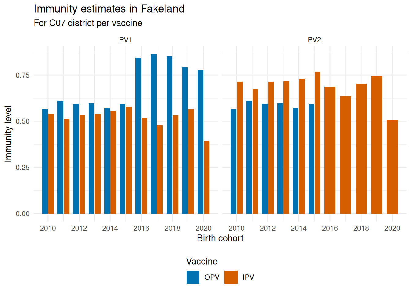
Immunity levels generally track with vaccine efficacy (see the efficacy table below) and coverage levels (see Section 4.3). In this example using two doses of IPV and OPV, both tOPV (pre-2016) and bOPV (post-2016) exhibit higher efficacy against PV1 than IPV, which is reflected in the resulting immunity estimates. Conversely, IPV provides higher efficacy against PV2 than tOPV. Since bOPV does not target PV2, OPV-derived immunity for this serotype doesn’t have values after 2015. Additionally, the slightly higher dose counts for OPV compared to IPV seen in Section 4.3 further contribute to the observed differences in immunity levels.

efficacy

serotype	vaccine	vaccine_type	dose	efficacy	from	to
PV1	OPV	tOPV	OPV0	0.3900	NA	2015
PV1	OPV	tOPV	OPV1	0.6279	NA	2015
PV2	OPV	tOPV	OPV0	0.3900	NA	2015
PV2	OPV	tOPV	OPV1	0.6279	NA	2015
PV1	OPV	bOPV	OPV0	0.6300	2016	NA
PV1	OPV	bOPV	OPV1	0.8631	2016	NA
PV1	IPV	IPV	IPV1	0.3500	NA	NA
PV1	IPV	IPV	IPV2	0.6000	NA	NA
PV1	IPV	IPV	IPV3	0.8400	NA	NA
PV1	IPV	IPV	IPV4	0.9400	NA	NA
PV2	IPV	IPV	IPV1	0.4100	NA	NA
PV2	IPV	IPV	IPV2	0.8000	NA	NA
PV2	IPV	IPV	IPV3	0.9600	NA	NA
PV2	IPV	IPV	IPV4	0.9900	NA	NA

4.5 Immunity estimation by immunity type

While compute_immunity() estimates immunity levels by vaccine, the epidemiologically relevant metric is often the type of immunity conferred. Different vaccines provide distinct immune responses: for example, OPV confers both mucosal and humoral immunity, while IPV provides only humoral immunity.

The compute_immunity_by_type() function combines vaccine-level estimates into immunity-type estimates. This requires two key inputs:

4.5.1 Vaccine-immunity type mapping

The vax_imm_type argument specifies which immunity types each vaccine confers. This should be a named list where:

Keys: Vaccine names (e.g., “OPV”, “IPV”)
Values: Character vectors of immunity types (e.g., c("mucosal", "humoral"))

Default for polio vaccines: If you are working exclusively with OPV and IPV, you can omit this argument. The function defaults to:

list(OPV = c("mucosal", "humoral"), IPV = "humoral")

Flexibility: The function accommodates any number of immunity types and vaccine combinations, provided that (1) the immunity types are specified in vax_imm_type, and (2) the corresponding vaccine doses appear in both your routine immunization data and efficacy estimates.

4.5.2 Correlation between vaccines

The rho argument controls the correlation between different vaccines when calculating immunity at the population level. This parameter is crucial when multiple vaccines contribute to the same immunity type:

rho = 0: Assumes that receiving one vaccine is unrelated to receiving another vaccine.
rho = 1: Assumes that children who receive one vaccine are as likely as possible to also receive the other vaccine.
0 < rho < 1: Assumes partial correlation, indicating some level of association between vaccine uptake.

If more than two vaccines contribute to the same immunity type, rho might be:

a single value applied uniformly across all vaccine pairs, or
a correlation matrix specifying pairwise correlations between each vaccine.

This parameter represents assumptions about the overlap in uptake of vaccines that confer the same immunity type. The calculation applies this assumption when combining vaccine-specific immunity estimates.

The function validate_vax_imm_type() can be used to check that the vax_imm_type argument is correctly specified and consistent with the vaccines present in your data.

For detailed documentation, run ?compute_immunity_by_type. The code snippet below shows how to use this function:

immunity_by_type <- compute_immunity_by_type(
  immunity,
  vax_imm_type = vaccine_immunity_type,
  rho = 0 # No correlation
) %>%
  mutate(type = factor(type, levels = c("mucosal", "humoral")))

head(immunity_by_type, 10)

prov_code	dist_code	year	serotype	type	immunity_level	live_births
PR_C	C05	2013	PV1	humoral	0.8278725	58294
PR_D	D05	2015	PV1	humoral	0.8325977	43460
PR_F	F03	2017	PV1	humoral	0.9238353	39924
PR_C	C05	2014	PV1	humoral	0.8161490	60063
PR_D	D07	2016	PV1	humoral	0.9379865	50585
PR_B	B02	2012	PV1	humoral	0.8182312	35587
PR_A	A03	2017	PV1	humoral	0.9423444	51241
PR_C	C02	2020	PV1	humoral	0.8943612	54672
PR_E	E03	2010	PV1	humoral	0.8388713	51252
PR_F	F01	2018	PV1	humoral	0.9063387	36763

immunity_by_type %>%
  filter(dist_code == .dcode) %>%
  ggplot(aes(
    x = year,
    y = immunity_level,
    fill = factor(type, levels = c("mucosal", "humoral"))
  )) +
  geom_col(position = "dodge2", width = 0.8) +
  facet_grid(~serotype) +
  scale_x_continuous(breaks = scales::breaks_width(2)) +
  scale_fill_manual(
    name = "Immunity type",
    values = imm_color_scheme
  ) +
  guides(
    fill = guide_legend(nrow = 1, byrow = TRUE, title.position = "top"),
    alpha = guide_legend(nrow = 1, byrow = TRUE, title.position = "top")
  ) +
  theme_minimal() +
  theme(legend.position = "bottom", legend.box = "horizontal") +
  labs(
    title = "Immunity estimates in Fakeland",
    subtitle = sprintf("For %s district per immunity type", .dcode),
    x = "Birth cohort",
    y = "Immunity level"
  )

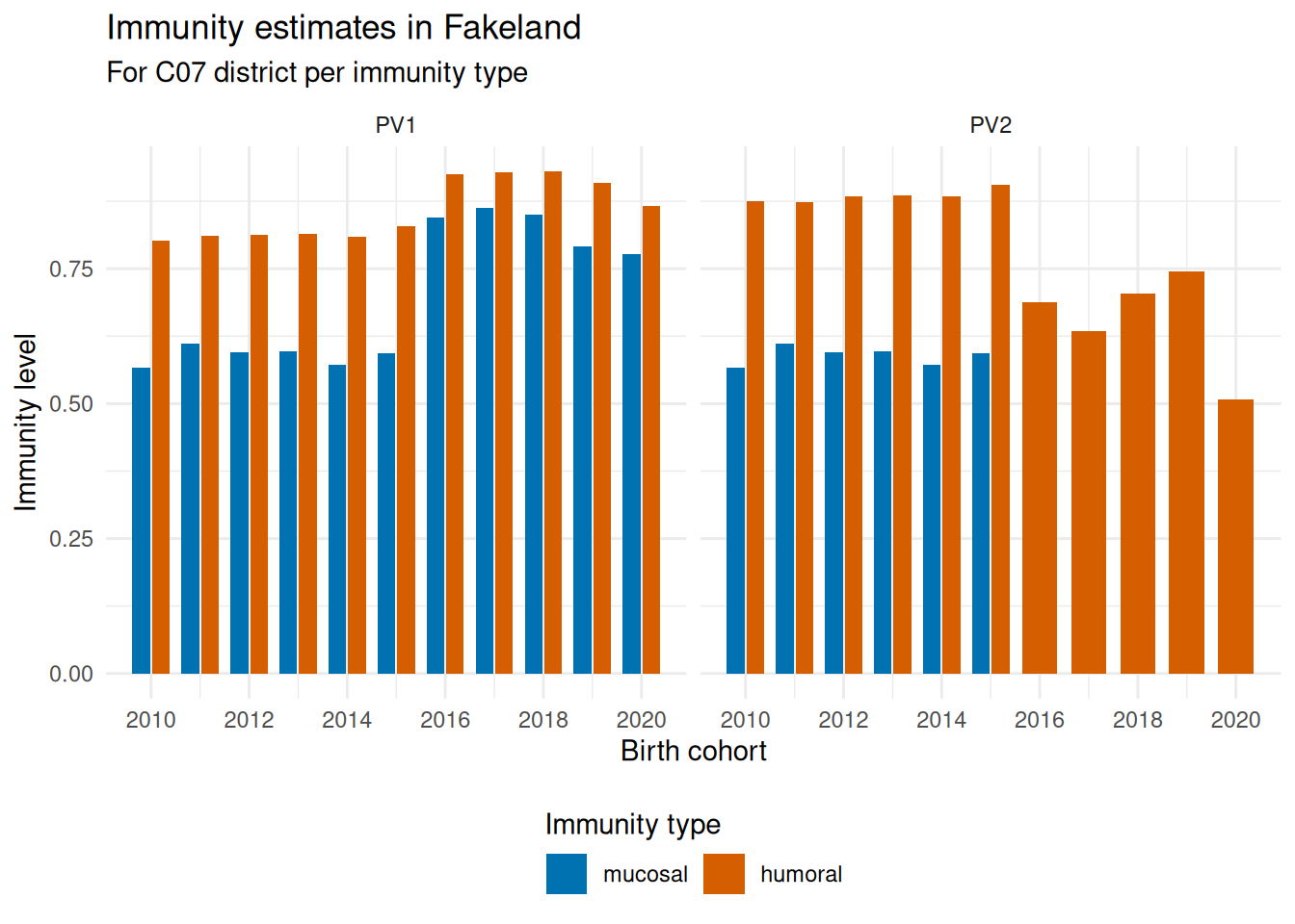
Here, humoral immunity levels are generally higher than mucosal immunity levels. This is expected because both OPV and IPV contribute to humoral immunity, whereas only OPV contributes to mucosal immunity. The decline in humoral immunity for PV2 after 2015 reflects the switch from tOPV to bOPV, which removed the PV2 component from the vaccine schedule. Accordingly, mucosal immunity for PV2 is not estimated after 2015.

4.6 Wrapper functions

The pviem package provides three convenience functions that execute the entire pipeline described above in a streamlined workflow:

compute_immunity_sample(): Executes all steps from imputation through immunity estimation for a single imputation sample. Users can choose vaccine-level estimates or combine vaccines by immunity type using per_imm_type.
compute_immunity_samples(): Performs the complete process across multiple imputation samples. The number of samples depends on your chosen imputation mode:
- ‘deterministic’: Fixed at 3 samples (minimum, mean, and maximum aggregations)
- ‘stochastic’: User-specified via the n_samples argument
- ‘custom’: Specify n_samples if your custom function is stochastic; otherwise, all samples will yield identical results
summarize_immunity_samples(): Aggregates estimates across samples. .lower and .upper are empirical 2.5% and 97.5% quantiles and describe the distribution across imputation samples. .ci95l and .ci95u are t-based confidence limits for the sample mean and answer a different question.

4.6.1 Performance optimization

To enable parallel processing of multiple samples, follow the installation instructions in vignette("setup") for configuring the necessary dependencies.

For complete documentation on these functions, run ?compute_immunity_samples.

4.6.2 One sample immunity estimation

immunity_1 <- compute_immunity_sample(
  ri_data = ri_data,
  efficacy = efficacy,
  neighbors = neighbors,
  vs_info = vs_table,
  birth_seasonality = birth_seasonality,
  sample_pair = sample_pair,
  imputation_mode = "stochastic",
  sample_mode = "gaussian",
  bandwidth = 1.0, # Only used if sample_mode is "gaussian"
  zero.rm = TRUE,
  shift_mode = "full",
  hed_assumption = "redistribute",
  max_level = 4,
  dd_assumption = "organised",
  vax_imm_type = vaccine_immunity_type,
  rho = 0,
  per_imm_type = TRUE, # Per immunity type estimates not vaccine
  quiet = TRUE
) %>%
  mutate(type = factor(type, levels = c("mucosal", "humoral")))

head(immunity_1, 10)

prov_code	dist_code	year	serotype	type	immunity_level	live_births
PR_C	C03	2010	PV1	humoral	0.8094682	41040
PR_C	C01	2011	PV1	humoral	0.8185671	44126
PR_B	B06	2020	PV1	humoral	0.8787726	38005
PR_C	C03	2015	PV1	humoral	0.8397119	42156
PR_C	C02	2012	PV1	humoral	0.8434337	55353
PR_C	C02	2017	PV1	humoral	0.9224829	55646
PR_B	B01	2017	PV1	humoral	0.9365669	52437
PR_F	F01	2020	PV1	humoral	0.8670189	36331
PR_B	B01	2016	PV1	humoral	0.9165385	52281
PR_C	C01	2010	PV1	humoral	0.8252044	42295

immunity_1 %>%
  filter(dist_code == .dcode) %>%
  ggplot(aes(
    x = year,
    y = immunity_level,
    fill = factor(type, levels = c("mucosal", "humoral"))
  )) +
  geom_col(position = position_dodge(width = 0.9), width = 0.8) +
  facet_grid(~serotype) +
  scale_x_continuous(breaks = scales::breaks_width(2)) +
  scale_fill_manual(name = "Immunity type", values = imm_color_scheme) +
  guides(
    fill = guide_legend(nrow = 1, byrow = TRUE, title.position = "top"),
    alpha = guide_legend(nrow = 1, byrow = TRUE, title.position = "top")
  ) +
  theme_minimal() +
  theme(legend.position = "bottom", legend.box = "horizontal") +
  labs(
    title = "Immunity estimates in Fakeland using one imputation sample",
    subtitle = sprintf("For %s district per immunity type", .dcode),
    x = "Birth cohort",
    y = "Immunity level"
  )

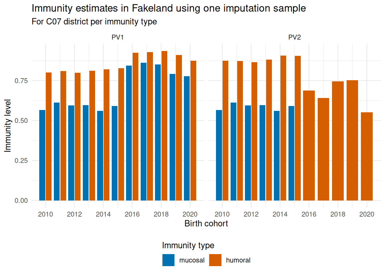
This result can be interpreted as in Section 4.5.

4.6.3 Summarized multiple samples immunity estimation

immunity_n <- compute_immunity_samples(
  n_samples = 5,
  ri_data = ri_data,
  vs_info = vs_table,
  efficacy = efficacy,
  birth_seasonality = birth_seasonality,
  neighbors = neighbors,
  sample_pair = sample_pair,
  imputation_mode = "stochastic",
  sample_mode = "uniform",
  # bandwidth = 1.0, # Only used if sample_mode is "gaussian"
  zero.rm = TRUE,
  shift_mode = "full",
  hed_assumption = "redistribute",
  max_level = 4,
  dd_assumption = "organised",
  vax_imm_type = vaccine_immunity_type,
  rho = 0,
  per_imm_type = TRUE,
  quiet = TRUE,
  seed = seed
)
head(immunity_n, 10)

prov_code	dist_code	year	serotype	type	immunity_level	live_births	sample
PR_F	F03	2011	PV1	humoral	0.8320172	39340	1
PR_C	C04	2014	PV1	humoral	0.8493318	59541	1
PR_D	D02	2014	PV1	humoral	0.8219921	51452	1
PR_F	F03	2016	PV1	humoral	0.9073692	39211	1
PR_A	A05	2010	PV1	humoral	0.8094095	51406	1
PR_C	C05	2019	PV1	humoral	0.9067875	58510	1
PR_A	A08	2012	PV1	humoral	0.8396021	36922	1
PR_A	A01	2017	PV1	humoral	0.9234168	42093	1
PR_E	E04	2012	PV1	humoral	0.8345545	41213	1
PR_A	A01	2014	PV1	humoral	0.8394617	42742	1

Five samples keep this example fast but are not enough for stable tail quantiles. In a real analysis, increase n_samples until the summary estimates and intervals are stable.

4.6.4 District level

immunity_dist <- immunity_n %>%
  summarize_immunity_samples() %>%
  mutate(type = factor(type, levels = c("mucosal", "humoral")))

head(immunity_dist, 10)

prov_code	dist_code	year	serotype	type	.mean	.sd	.median	.lower	.upper	.ci95l	.ci95u
PR_F	F03	2011	PV1	humoral	0.8267057	0.0034429	0.8247088	0.8239099	0.8316492	0.8224308	0.8309807
PR_C	C04	2014	PV1	humoral	0.8493411	0.0000127	0.8493430	0.8493261	0.8493565	0.8493253	0.8493569
PR_D	D02	2014	PV1	humoral	0.8223947	0.0003969	0.8224044	0.8220055	0.8229636	0.8219019	0.8228876
PR_F	F03	2016	PV1	humoral	0.9046483	0.0026193	0.9057230	0.9017938	0.9072769	0.9013960	0.9079005
PR_A	A05	2010	PV1	humoral	0.8063637	0.0072310	0.8094095	0.7983127	0.8127033	0.7973852	0.8153422
PR_C	C05	2019	PV1	humoral	0.9072122	0.0007337	0.9071548	0.9064349	0.9082451	0.9063011	0.9081232
PR_A	A08	2012	PV1	humoral	0.8419114	0.0017766	0.8431935	0.8396794	0.8431935	0.8397054	0.8441174
PR_A	A01	2017	PV1	humoral	0.9228570	0.0008005	0.9231387	0.9218252	0.9236481	0.9218630	0.9238510
PR_E	E04	2012	PV1	humoral	0.8279406	0.0064814	0.8248625	0.8209580	0.8349543	0.8198929	0.8359883
PR_A	A01	2014	PV1	humoral	0.8398836	0.0008902	0.8395847	0.8392622	0.8412718	0.8387782	0.8409890

immunity_dist %>%
  filter(dist_code == .dcode) %>%
  ggplot(aes(
    x = year,
    y = .mean,
    ymin = .lower,
    ymax = .upper,
    fill = factor(type, levels = c("mucosal", "humoral"))
  )) +
  geom_col(position = position_dodge(width = 0.9)) +
  geom_errorbar(
    position = position_dodge(width = 0.9),
    width = 0.4,
  ) +
  facet_grid(~serotype) +
  scale_x_continuous(breaks = scales::breaks_width(2)) +
  scale_fill_manual(name = "Immunity type", values = imm_color_scheme) +
  guides(
    fill = guide_legend(nrow = 1, byrow = TRUE, title.position = "top"),
    alpha = guide_legend(nrow = 1, byrow = TRUE, title.position = "top")
  ) +
  theme_minimal() +
  theme(legend.position = "bottom", legend.box = "horizontal") +
  labs(
    title = "Immunity estimates in Fakeland for multiple samples",
    subtitle = sprintf(
      "For %s district per immunity type with an empirical 95%% interval",
      .dcode
    ),
    x = "Birth cohort",
    y = "Immunity level"
  )

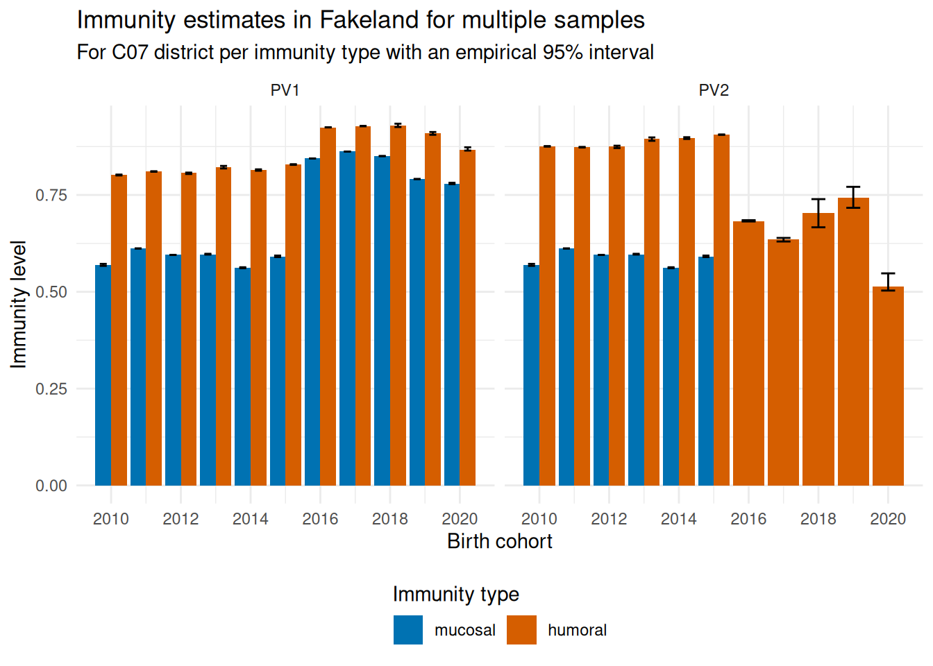
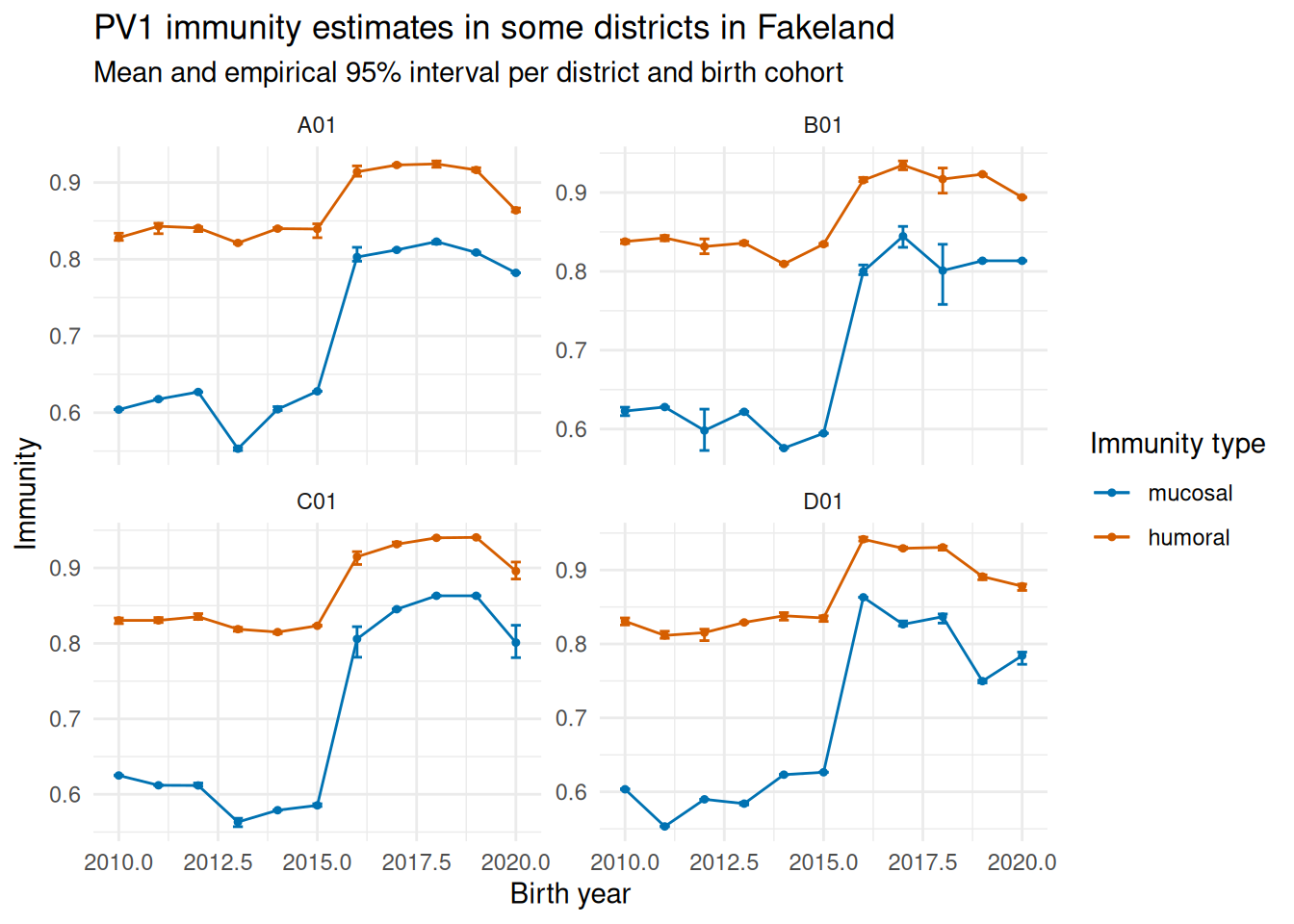
This plot shows the mean estimate and the empirical interval from the 2.5% to 97.5% sample quantiles. A wider interval indicates greater variation across imputation samples, which may reflect uncertainty arising from missing data and the selected model assumptions.

immunity_dist[
  dist_code %in%
    c('A01', 'B01', 'C01', 'D01') &
    serotype == serotype_eg,
] |>
  ggplot(aes(x = year, y = .mean, ymin = .lower, ymax = .upper, color = type, fill = type)) +
  geom_line() +
  geom_point(size = .9) +
  # geom_ribbon(alpha = alpha_, color = NA) +
  geom_errorbar(width = 0.25) +
  facet_wrap(~dist_code, scales = "free_y") +
  scale_color_manual(values = imm_color_scheme) +
  scale_fill_manual(values = imm_color_scheme) +
  theme_minimal() +
  labs(
    title = sprintf(
      "%s immunity estimates in some districts in Fakeland",
      serotype_eg
    ),
    subtitle = "Mean and empirical 95% interval per district and birth cohort",
    x = "Birth year",
    y = "Immunity",
    color = "Immunity type",
    fill = "Immunity type"
  )

4.6.5 Province level

immunity_prov <- immunity_n %>%
  summarize_immunity_samples(by_admin = "prov_code") %>%
  mutate(type = factor(type, levels = c("mucosal", "humoral")))

head(immunity_prov, 10)

prov_code	year	serotype	type	.mean	.sd	.median	.lower	.upper	.ci95l	.ci95u
PR_F	2011	PV1	humoral	0.8317052	0.0087331	0.8275144	0.8209752	0.8440216	0.8276180	0.8357924
PR_C	2014	PV1	humoral	0.8200993	0.0184905	0.8161979	0.7861167	0.8493494	0.8137476	0.8264510
PR_D	2014	PV1	humoral	0.8176770	0.0153878	0.8224044	0.7856410	0.8414530	0.8130540	0.8223000
PR_F	2016	PV1	humoral	0.9240966	0.0139171	0.9262625	0.9018481	0.9387131	0.9175832	0.9306100
PR_A	2010	PV1	humoral	0.8226061	0.0104477	0.8250545	0.7997343	0.8374451	0.8194673	0.8257450
PR_C	2019	PV1	humoral	0.9288427	0.0142082	0.9378124	0.9062157	0.9417388	0.9239620	0.9337234
PR_A	2012	PV1	humoral	0.8370207	0.0070547	0.8393857	0.8174550	0.8451526	0.8349013	0.8391402
PR_A	2017	PV1	humoral	0.9199386	0.0177892	0.9217745	0.8912850	0.9429963	0.9145941	0.9252831
PR_E	2012	PV1	humoral	0.8243528	0.0098783	0.8258598	0.8042737	0.8373008	0.8202752	0.8284303
PR_A	2014	PV1	humoral	0.8319115	0.0125608	0.8363136	0.8080841	0.8470977	0.8281378	0.8356851

# Retrieve province code for the example district
.pcode <- immunity_dist %>%
  filter(dist_code == .dcode) %>%
  pull(prov_code) %>%
  unique()

immunity_prov %>%
  filter(prov_code == .pcode) %>%
  ggplot(aes(
    x = year,
    y = .mean,
    ymin = .lower,
    ymax = .upper,
    fill = factor(type, levels = c("mucosal", "humoral"))
  )) +
  geom_col(position = position_dodge(width = 0.9)) +
  geom_errorbar(
    position = position_dodge(width = 0.9),
    width = 0.4,
  ) +
  facet_grid(~serotype) +
  scale_x_continuous(breaks = scales::breaks_width(2)) +
  scale_fill_manual(name = "Immunity type", values = imm_color_scheme) +
  guides(
    fill = guide_legend(nrow = 1, byrow = TRUE, title.position = "top"),
    alpha = guide_legend(nrow = 1, byrow = TRUE, title.position = "top")
  ) +
  theme_minimal() +
  theme(legend.position = "bottom", legend.box = "horizontal") +
  labs(
    title = "Immunity estimates in Fakeland using multiple imputation samples",
    subtitle = sprintf("For %s province per immunity type with an empirical 95%% interval", .pcode),
    x = "Birth cohort",
    y = "Immunity level"
  )

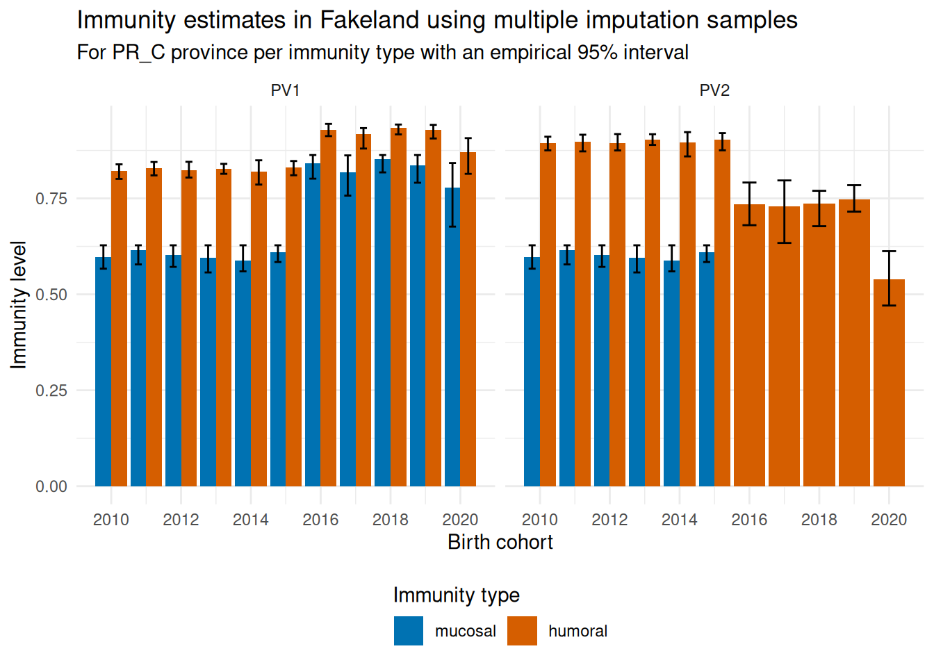
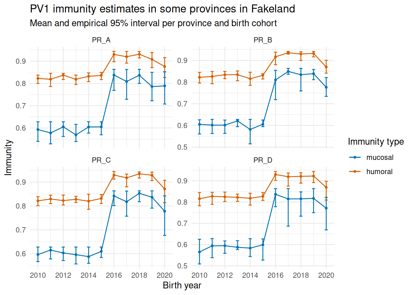
This plot shows the same information as the previous plot, but at the province level.

immunity_prov[
  prov_code %in%
    c('PR_A', 'PR_B', 'PR_C', 'PR_D') &
    serotype == serotype_eg,
] |>
  ggplot(aes(x = year, y = .mean, ymin = .lower, ymax = .upper, color = type, fill = type)) +
  geom_line() +
  geom_point(size = .9) +
  # geom_ribbon(alpha = alpha_, color = NA) +
  geom_errorbar(width = 0.25) +
  facet_wrap(~prov_code, scales = "free_y") +
  scale_x_continuous(breaks = scales::breaks_width(2)) +
  scale_color_manual(values = imm_color_scheme) +
  scale_fill_manual(values = imm_color_scheme) +
  theme_minimal() +
  labs(
    title = sprintf("%s immunity estimates in some provinces in Fakeland", serotype_eg),
    subtitle = "Mean and empirical 95% interval per province and birth cohort",
    x = "Birth year",
    y = "Immunity",
    color = "Immunity type",
    fill = "Immunity type"
  )

5 Migration from version 0.1.x to 0.2.x

If you are migrating from version 0.1.x to 0.2.0, please note the following breaking changes:

The package now requires R >= 4.4.0.
Use config_pviem() to set global configuration options especially for column names in your dataset. This function allows you to specify the column names for live births, administrative levels, time, and other key variables, ensuring that the package functions can correctly identify and process your data.
Birth seasonality birth column name has changed from births to the column name specified in the birth argument of config_pviem(), which defaults to live_births to have a consistent naming convention across datasets.
get_default_sample_pair() function signature has changed.
Optional arguments (arguments with default values) in all functions should now be named. For example, instead of compute_immunity(ri_data, efficacy, "organised"), you should now use compute_immunity(ri_data, efficacy, dd_assumption = "organised"). This change was made to improve code readability and reduce the likelihood of errors when using functions with many arguments. We recommend using named arguments for all function calls to enhance clarity, even for required arguments.
There are several deprecations the user will need to address when migrating to version 0.2.0, which are detailed in the documentation of the respective functions.

6 Future potential improvements

The current implementation of the pviem package provides a solid foundation for estimating polio immunity levels. However, several enhancements could further improve the package’s functionality and scope:

6.1 Supplementary immunization activities (SIAs)

The current version does not incorporate supplementary immunization activities (SIAs)—mass vaccination campaigns conducted outside routine immunization schedules. SIAs play a critical role in polio eradication efforts, particularly in outbreak response and campaign settings. Including SIA data would provide a more complete picture of population immunity.

Proposed enhancement: Extend the package to accept SIA datasets as optional inputs, allowing the immunity estimation pipeline to account for both routine immunization and campaign-based coverage when calculating immunity levels.

6.2 Overlapping vaccination schedules

The current implementation assumes non-overlapping vaccination periods for different vaccine types within the same vaccine family. For instance, with OPV vaccines, the package assumes that trivalent OPV (tOPV) and bivalent OPV (bOPV) are used in distinct, non-overlapping time periods.

However, this assumption does not always hold in practice. Many countries experienced transition periods where multiple OPV formulations were used concurrently—particularly during the global switch from tOPV to bOPV. During these transitions, districts or vaccination sites may have administered both vaccine types simultaneously.

Proposed enhancement: Extend the package to handle overlapping vaccination schedules by:

Allowing users to specify time periods for each vaccine type with potential overlaps
Implementing allocation rules when multiple vaccine types are administered in the same year
Adjusting immunity calculations to account for children who may have received mixed vaccine schedules

This would better reflect real-world vaccination programs and improve accuracy during vaccine transition periods.